Today, we talk about the Passive Intermodulation PIM in Base Stations, Passive Intermodulation PIM’s challenges, and solutions.
Active devices are known to produce nonlinear effects in systems. Various techniques have been developed to improve the performance of such devices during the design and operation phases. It is easy to overlook that passive device may also introduce nonlinear effects; although sometimes relatively small, these nonlinear effects can seriously affect system performance if left uncorrected.
PIM indicates passive intermodulation. It represents the cross-modulation product generated when two or more signals are transmitted through a passive device with nonlinear characteristics.
The interaction of mechanically connected parts generally causes nonlinear effects, which are particularly evident at the joints of two different metals. Examples include loose cable connections, unclean connectors, poorly performing duplexers, or aging antennas.
Passive cross-modulation is a major problem in the cellular communications industry and is very difficult to troubleshoot. In cellular communication systems, PIM can cause interference, reduce receiver sensitivity, or even block communications all together. This interference can affect the cell that generates it as well as other receivers in the vicinity.
For example, in LTE band 2, the downlink range is 1930 MHz to 1990 MHz and the uplink range is 1850 MHz to 1910 MHz. If two transmitting carriers located at 1940 MHz and 1980 MHz respectively transmit signals from a base station system with PIM, their intermodulation will produce a component located at 1900 MHz This component falls into the receive band, which affects the receiver. In addition, the intermodulation located at 2020 MHz may affect other systems.
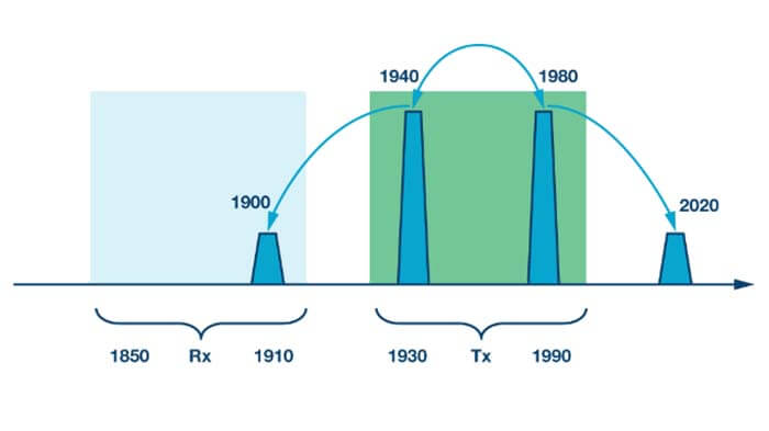
Figure1 Passive intermodulation PIM falling into the receiver band
As the spectrum becomes more crowded and antenna sharing schemes become more common, the possibility of PIM from intermodulation of different carriers is increasing. Traditional methods of using frequency planning to avoid PIM are becoming less and less feasible.
In addition to these challenges, the adoption of new digital modulation schemes such as CDMA/OFDM means that the peak power of communications systems is also increasing, making the PIM problem even more severe.
For service providers and equipment vendors, PIM is a prominent and serious problem. Detecting and, where possible, solving the problem can improve system reliability and reduce operating costs. This paper attempts to review the sources and causes of PIM, as well as techniques to detect and resolve it.
Passive intermodulation PIM classification
Preliminary investigation shows that there are three different types of PIM, each with different characteristics and requiring different solutions. We have chosen to classify them according to the following types, design introduction PIM, assembly PIM, and rust body PIM.
Design to introduce PIM
We know that certain passive devices along with their transmission lines produce passive cross-tuning. Therefore, when designing a system, the development team should select passive components with minimal or acceptable levels of PIM according to the specifications given by the device manufacturer.
Circulators, duplexers, and switches are particularly susceptible to PIM effects. Designers who can accept a higher level of passive cross-tuning then can choose lower cost, smaller size, or lower performance of the device.
Figure2 Device design trade-offs, size, power consumption, rejection, and PIM performance
If the designer does choose a lower performance device, the corresponding higher level of cross-tuning may fall back into the receiver band, resulting in receiver desensitization.
In this case, undesirable spectrum radiation or power efficiency loss may not be as much of a concern as PIM leading to receiver desensitization. This issue is particularly important in small cellular radio designs.
ADI is currently developing technology that can detect, simulate, and eliminate (offset) static passive components such as duplexers from the received signal PIM (see Figure 3).
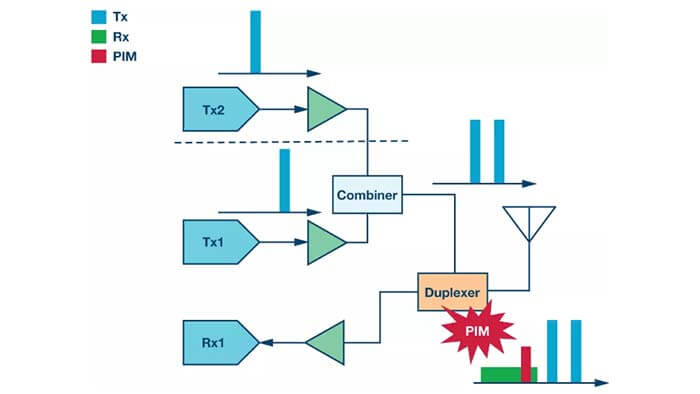
Figure3 Passive intermodulation PIM generation and PIM offset algorithm
The algorithm is effective because it is aware of the carrier information and can use receiver correlation to determine cross modulation artifacts, which can then be eliminated from the received signal.
The limitations of the algorithm begin to emerge when the correlation can no longer be used to determine cross modulation artifacts. Figure 4 shows an example. In this example, two different transmitters share a single antenna.
If the baseband processing of each path is assumed to be independent of each other, it is unlikely that the algorithm will be aware of both, and therefore it is limited in the correlation and offset processing it can perform at the receivers.
Figure4 Multiple sources share an antenna
The complexity of the Passive intermodulation PIM challenge
Site access and cost to service providers poses a challenge, we are beginning to find more and more such instances: different transmitters share a single broadband antenna. The architecture can be a mix of bands and formats: TDD + FDD; TDD: F + A + D, FDD: B3, etc.
Figure 5 shows an overview of this configuration. In this example, the customer is trying to implement a complex but realistic configuration. One branch is TDD dual-band and the other is FDD single-band with a single duplexer. The signals converge and share a single antenna. passive cross modulation between the Tx1 and Tx2 signals occurs in the path from the combiner, in the transmission line to the antenna, and in the antenna itself. The resulting cross modulation artifacts fall back to the FDD receiver band Rx2.
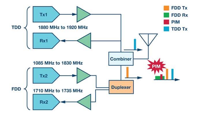
Figure 5 FDD/TDD single antenna implementation scheme
Practical analysis of a dual-band system is shown in Figure 6. Note that in this example, we need to consider passive modulation artifacts of more than third order. In this case, the focus is on the cross-modulation artifacts falling back from one band (internal) into the other receiver band.
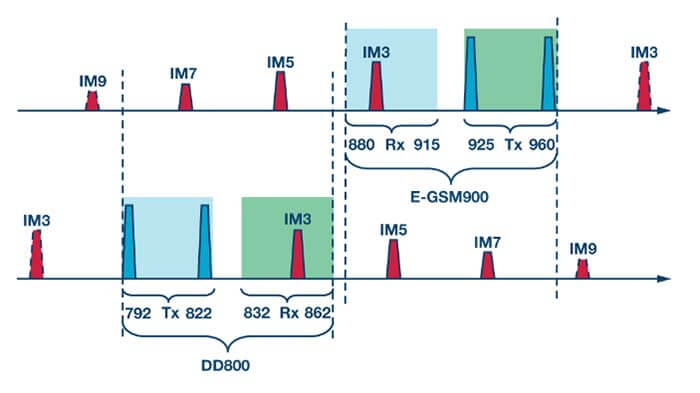
Figure6 Multi-frequency Passive intermodulation PIM problem
Assembly Passive intermodulation PIM
We call the second type of PIM assembly Passive intermodulation PIM. although the system can operate satisfactorily after installation, after a period of time, due to weather or poor quality of the initial installation, its performance often degrades.
When this happens, the passive components in the signal path (connectors, cables, cable assemblies, waveguide assemblies, components, etc.) typically begin to exhibit nonlinear behavior. In fact, some of the major PIM phenomena are caused by connectors, connections, and even the feed line of the antenna itself.
The resulting effects may be similar to the design-induced PIM discussed above, so the same PIM measurement theory can be used, which is specifically designed to look for the presence of passive cross-modulation products.
Typical factors that cause assembly Passive intermodulation PIM are as below.
Connector adaptation interface (usually N-type or DIN7/16)
Cable attachment (mechanical stability of the cable/connector bond)
Materials (brass and copper are recommended, ferromagnetic materials have non-linear properties)
Cleanliness (dust contamination or water vapor)
Cable factors (quality and robustness of the cable)
Mechanical robustness (wind and vibration-induced flexing)
Electro-thermal induction PIM (the cause is a non-constant envelope RF signal consuming power that varies with time, causing a change in temperature, which in turn causes a change in conductivity)
Environments with large temperature variations, salty/contaminated air, or the presence of excessive vibration tend to exacerbate PIM problems. Although the same PIM measurement techniques can be used for the design introduction of PIM, it can be assumed that the presence of assembly PIM indicates a reduction in both system performance and reliability.
If left unaddressed, the defective factors that cause PIM may intensify until the entire transmission path fails. The use of PIM offsetting methods for assembly PIM is more like covering up the problem than solving it.
In such cases, the user may not want to offset PIM but rather want to know the existence of PIM in order to eliminate the root cause. To do this, it is necessary to first determine where the PIM was introduced from the system and then repair or replace specific components.
We can consider the design introduction of PIM to be quantifiable and stable, but the assembly PIM described above is unstable. It may exist in a very narrow set of conditions with amplitude variations that may exceed 100 dB. A single offline scan may not capture such instances; ideally, transmission line diagnostics need to be performed in concert with PIM events.
Passive intermodulation PIM beyond the antenna (rusty PIM)
PIM is not limited to the wired transmission path, but may also occur outside the antenna. The effect is also known as rust PIM. in this case, passive cross-modulation occurs after the signal leaves the transmitter antenna, the resulting cross-modulation reflected back into the receiver.
The term rust body comes from the fact that in many cases, the intermodulation source may be rusted metal objects, such as wire mesh, warehouses, or drainpipes.
Metal objects can cause reflections. But in these cases, the metal object not only reflects the received signal but also generates and radiates intermodulation artifacts. Cross modulation occurs as in the wired signal path, i.e., at the interface of two different metals or heterogeneous materials.
The surface currents generated by the electromagnetic waves are mixed and re-radiated (see Figure 7). The amplitude of the re-radiated signal is generally very low. However, if the radiating object (rusty wire, warehouse or downpipe, etc.) is close to the base station receiver and the cross-modulation products fall within the receiver band, it will cause the receiver to be desensitized.
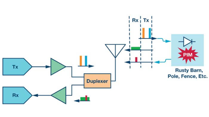
Figure 7 Outside the antenna or rusty body Passive intermodulation PIM
In some cases, the PIM source can be detected by antenna positioning: while changing the antenna position, while monitoring the PIM level. In addition, time delay estimation can also be used to locate the PIM source. If the PIM level is stable, standard algorithmic offset techniques can be used to compensate for PIM. but more often than not, the PIM contribution is affected by vibration, wind, and mechanical motion, making offsetting very difficult to perform.
Passive intermodulation PIM testing: locating PIM sources
Line Scanning
A variety of line scan techniques can be implemented. Line scan measures the signal loss and reflection of the transmission system over the target frequency band. We cannot assume that line scan will always accurately indicate the possible causes of PIM. A-line scan is more of a diagnostic tool that can help identify problems on the transmission line.
Early assembly problems may manifest as PIM; if left unresolved, these assembly problems may escalate and cause more serious transmission line failures.
Line scanning is usually divided into two basic tests, return loss and insertion loss. Both have a strong relationship with frequency, and both may vary greatly within the specified frequency band. Return loss measures the power transmission efficiency of the antenna system. Be sure to make the reflected power back to the transmitter is minimal. Any reflected power may distort the transmitted signal; if the reflected power is large enough, even damage the transmitter.
A return loss value of 20 dB means that 1% of the transmitted signal is reflected back to the transmitter and 99% reaches the antenna, which is usually considered to be a quite good performance. 10 dB of return loss means that 10% of the signal is reflected, indicating unsatisfactory performance. If the return loss measurement is 0 dB, then 100% of the power is reflected, which is most likely caused by an open or short circuit.
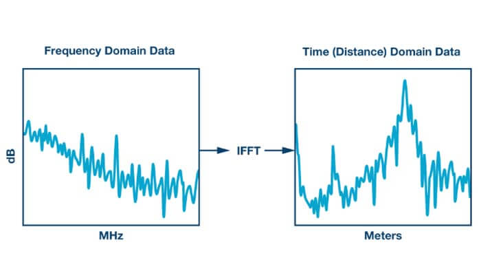
Time Domain Reflections
Advanced TDR techniques can be used to provide a reference mapping of the optimal system, as well as to determine the exact location on the transmission path where loss begins to occur. With this technique, the operator can locate the PIM source so that it can be repaired in a targeted and efficient manner.
Transmission line mapping also alerts the operator to some early signs of failure, preventing them from seriously affecting performance. Time-domain emission method (TDR) to measure the signal through the transmission line generated by the reflection. TDR instrument let a pulse through the medium, and then the unknown transmission environment generated by the reflection with the standard impedance generated by the reflection to compare. Figure 8 shows a simplified TDR measurement setup block diagram.
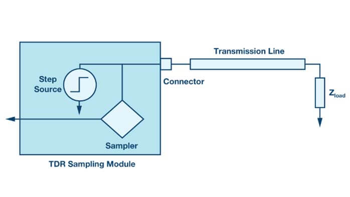
Figure 8 TDR setup block diagram
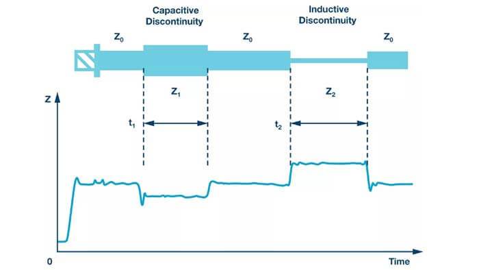
Figure 9 shows an example of a TDR transmission line mapping.
Frequency Domain Reflections
Although both TDR and FDR work by sending excitation signals along the transmission line and analyzing the reflections, the two techniques are implemented very differently. the FDR technique uses RF signal scanning instead of the DC pulses used in TDR.
In addition, FDR is much more sensitive than TDR and can locate areas of system performance failure or degradation with much higher accuracy. The principle of the frequency domain reflection method involves vector summation of the source and reflected signals (from faults and other reflected characteristics in the transmission line).
TDR uses very short DC pulses as the excitation signal, which inherently covers a very wide bandwidth, while FDR scans the RF signal is actually operating at a specific target frequency (usually within the expected operating range of the system).
Passive intermodulation PIM positioning
It must be noted that while a line scan can indicate an impedance mismatch and thus indicate a transmission line PIM source, PIM and transmission line impedance mismatch can be mutually exclusive.
PIM nonlinearity may occur where the line scan results do not indicate any transmission line problems. Therefore, to provide users with a solution that requires not only indicating the presence of PIM but also accurately identify where the problem occurs on the transmission line, a more complex implementation is required.
Comprehensive PIM line test works in a similar mode to that described for the design of the introduction of PIM offset, with the difference that the algorithm checks the cross-tuning product time delay estimates in different situations.
The priority in these cases is not the offset of PIM artifacts, but the location of where intermodulation occurs on the transmission line. This concept is also known as PIM localization(DTP). For example, in a two-tone test
Signal tone 1.
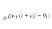
Signal tone 2.
w1 and w2 are the frequencies; θ1 and θ2 are the initial phases, and t0 is the initial time.
The IMD (e.g., low end) would be

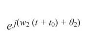
Many existing solutions require the user to interrupt the transmission path and insert a PIM standard device (which generates a fixed amount of PIM to calibrate the test equipment). Using a PIM standard device provides the user with a reference IMD that is at a specific location/distance of the transmission path and has a known phase. Figure 11(a) shows the overview. IMD phase θ32 (shown in Figure 11) is used as the reference position 0.
Fureig 11 PIM Positioning
Once the initial calibration is completed, the system is reconstructed and the system PIM is measured, as shown in Figure 11(b). the phase difference between θ32 and θ’32 can be used to calculate the distance to the PIM.
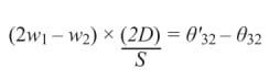
Where D is the distance to the PIM and S is the wave propagation velocity (depending on the transmission medium).
Assembly and rust PIM may be a slow and incremental process; initially, after completing the installation, the base station can work efficiently, but after a period of time, such PIM phenomena may start to become prominent. Environmental factors such as vibration or wind may affect PIM levels, so the nature and characteristics of PIM are dynamically fluctuating.
Masking or offsetting PIM may not only be difficult but may be perceived as masking more serious problems that, if left unaddressed, could trigger an overall system failure. In this case, operators will want to avoid the costs associated with overall system downtime by quickly locating the device causing the PIM and replacing it.
PIM location technology (DTP) also provides base station operators with the possibility of tracking system performance degradation over time to identify potential problems in advance. With this information, weak points can be replaced during planned maintenance, avoiding costly system downtime and specialized repair work.
Passive cross-tuning is nothing new. The phenomenon has been around for years and known for some time. In recent years, two different changes in the industry have brought it back into the limelight.
First, advanced algorithms can now detect and locate PIM in an intelligent way and can compensate for it as appropriate.
Previously, radio designers had to choose devices that could meet specific PIM performance requirements, but with the help of PIM offset algorithms, they now have greater freedom of choice.
They can choose to achieve higher performance or the same level of performance with lower cost and smaller devices. Offsetting algorithms digitally assist hardware components.
Second, as the density and diversity of base station towers explode, we face entirely new challenges from special system setups, such as antenna sharing.
Algorithmic offsets depend on knowledge of the main transmitted signals. In cases where space on the tower is valuable, different transmitters may share a single antenna, leading to a much higher likelihood of undesirable PIM effects.
In this case, the algorithm may know information about certain parts of the transmitter path and can work effectively. In the case where information about certain parts of the transmitter path is unknown, the performance or implementation of first-generation advanced PIM offset algorithms may be limited.
As the challenges in the area of base station equipment continue to become more difficult, PIM detection and offset algorithms are expected to provide considerable benefits and advantages to radio designers in the short term but require development efforts to keep pace with future challenges.
Besides the 10 Tips To Protect The IoT Security article, You may also be interested in the below articles.
What is the difference between WIFI and WLAN?
Summary of 41 Basic Knowledge of LTE
What Is The 5G Network Slicing?